Introducción a los SIG en R
Antonio J. Pérez-Luque 
Instituto de Ciencias Forestales (CIFOR) | INIA-CSIC (Madrid)
2025-02-07
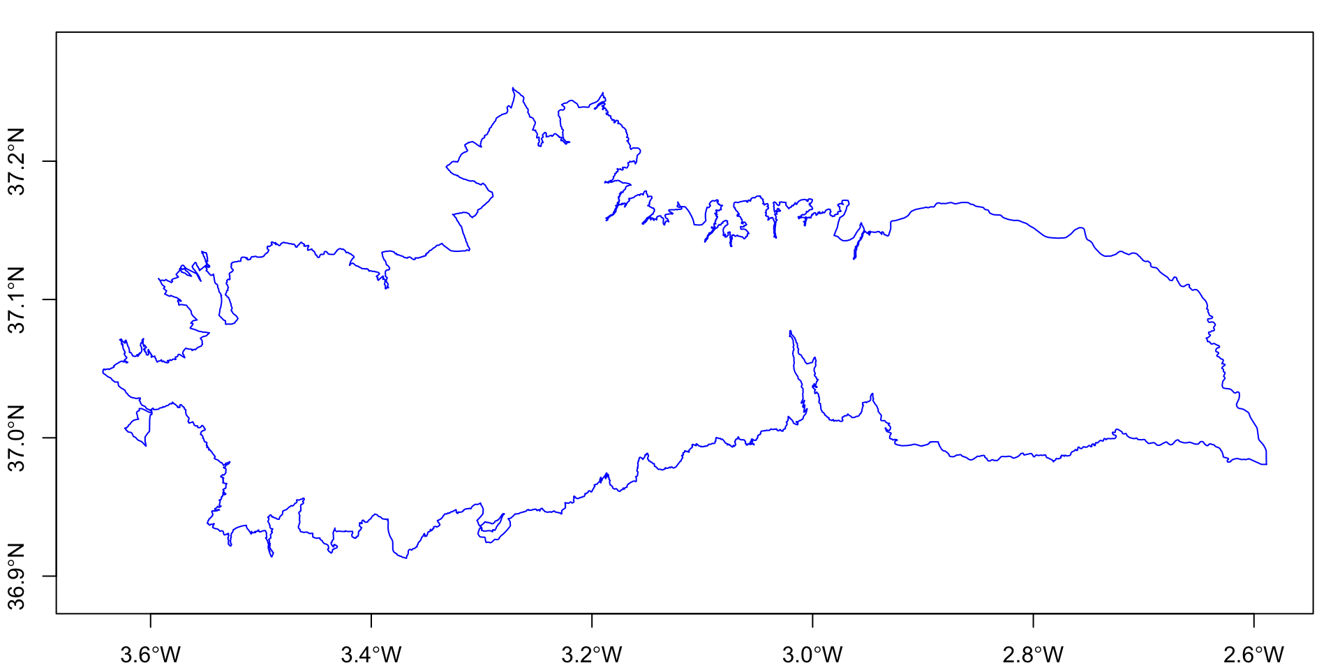
Datos Vectoriales
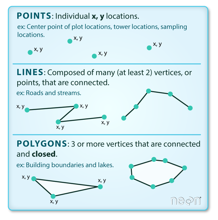
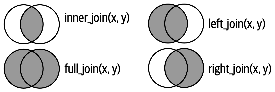
The big 7
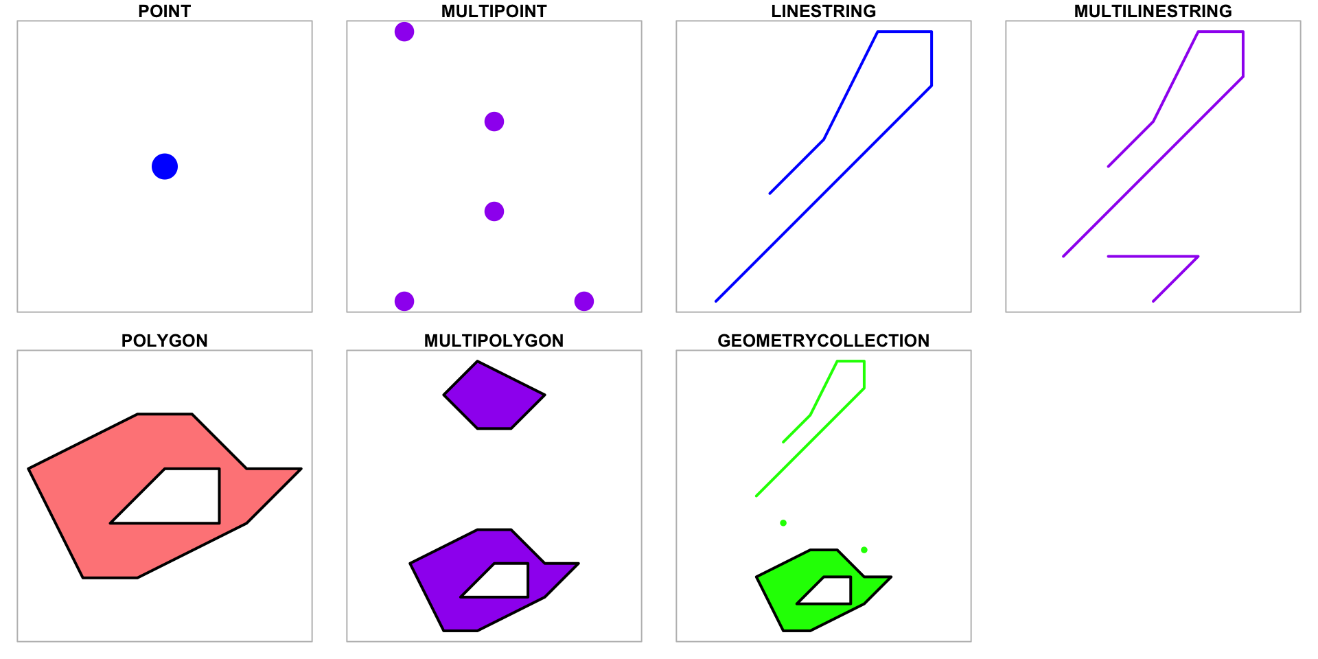
Simple feature geometries
- La representación en fomato texto se conoce como Well-Known Text (WKT)
MULTIPOLYGON (((2 1, 3 1, 5 2, 6 3, 5 3, 4 4, 3 4, 1 3, 2 1), (2.5 2, 3.5 3, 4.5 3, 4.5 2, 2.5 2)), ((3 7, 4 7, 5 8, 3 9, 2 8, 3 7)))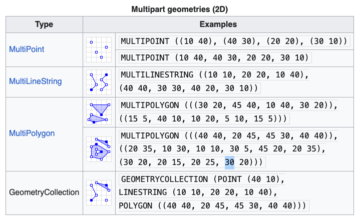
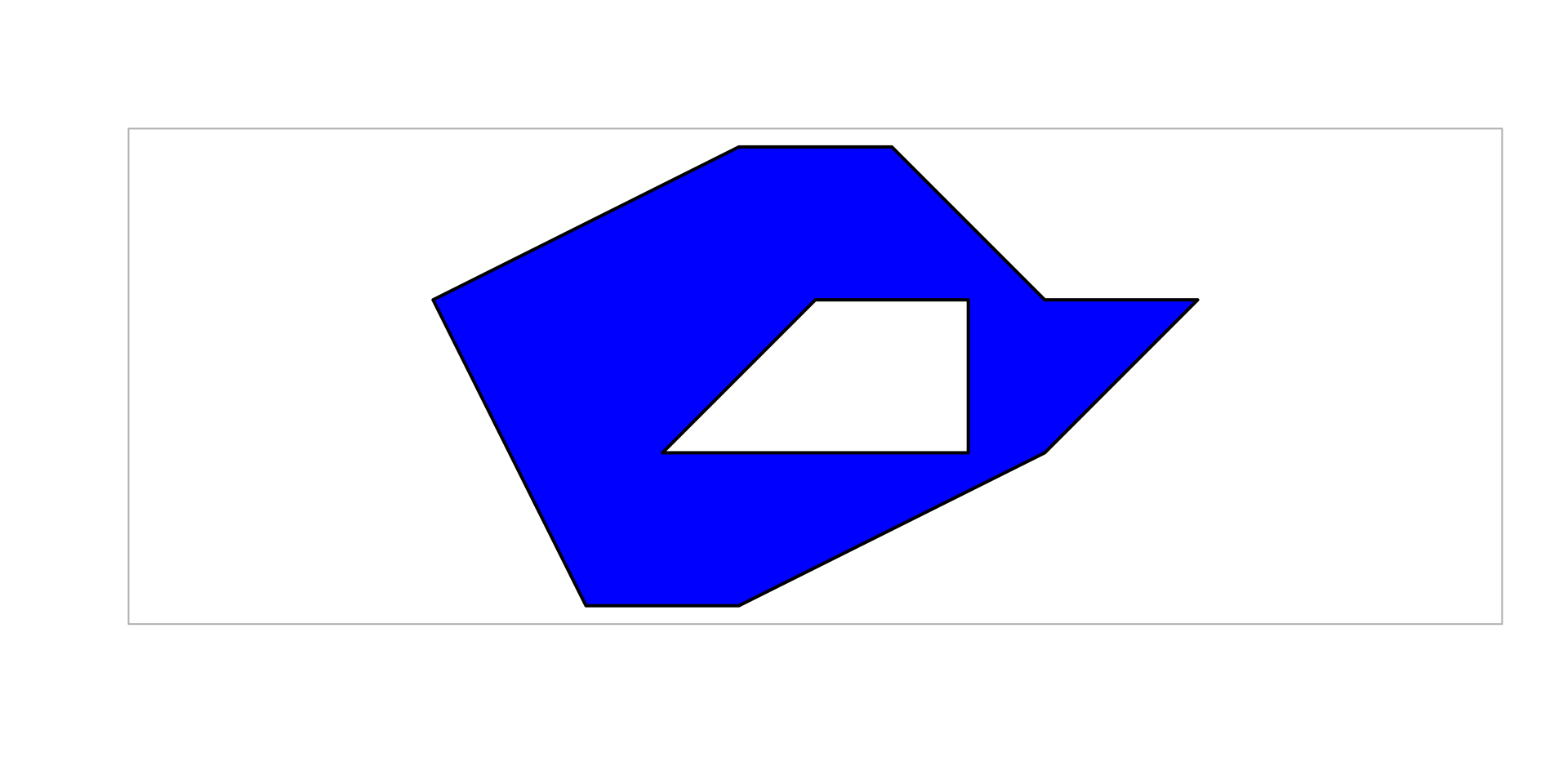
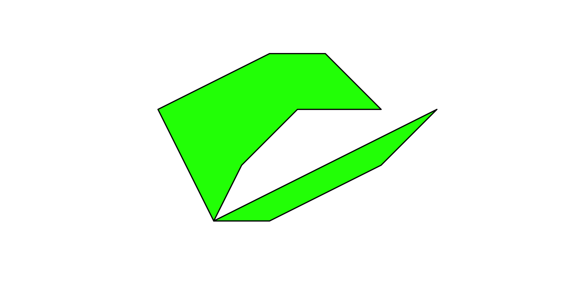
¿Geometrías válidas?
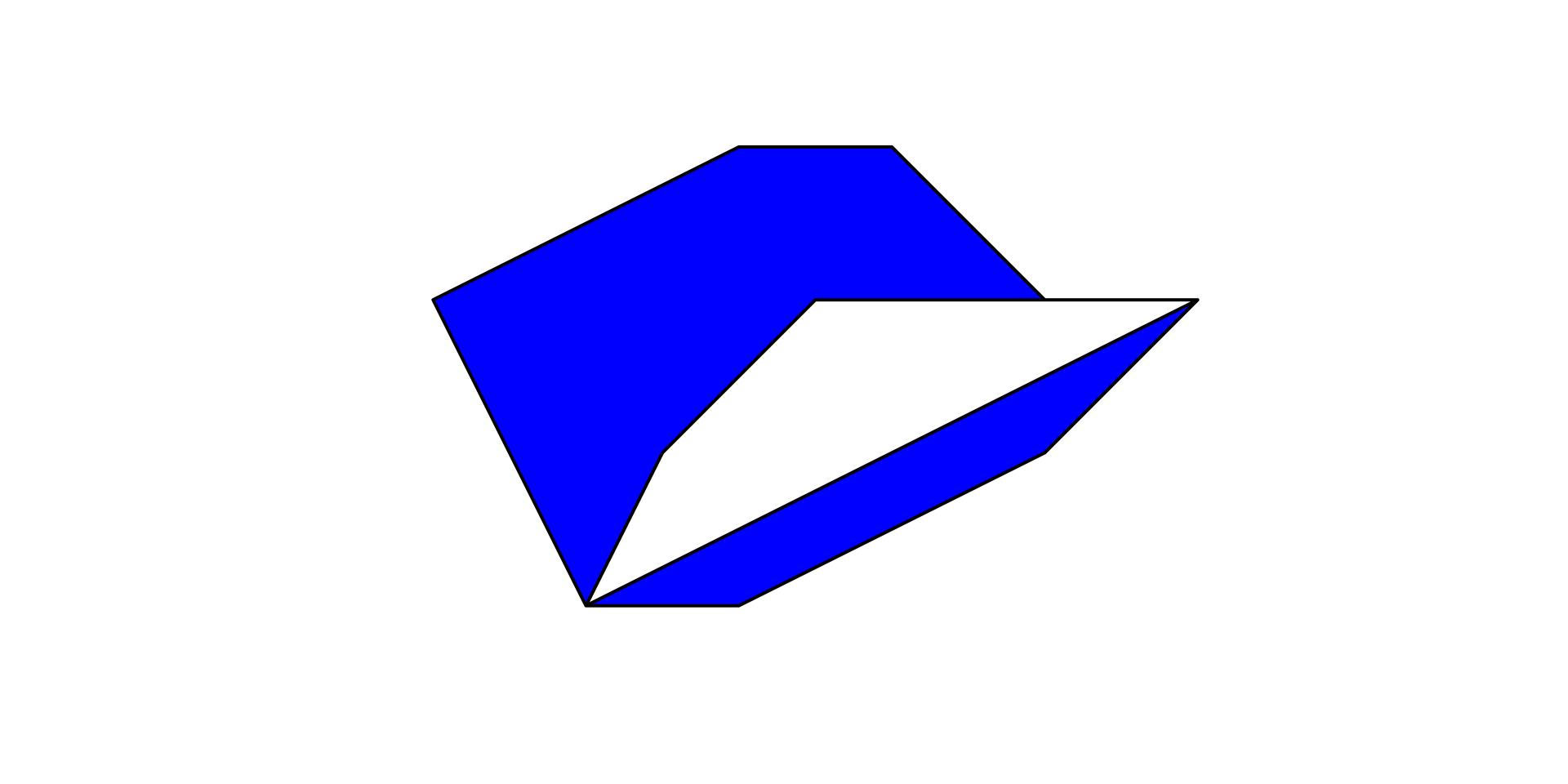
- Convertir a válido
Atributos (I)
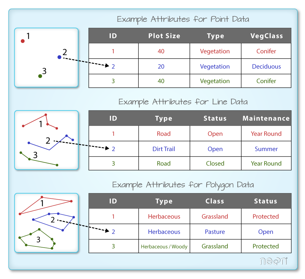
Atributos: derivados de geometría
Visualizar
Visualizar
Convertir a objetos spaciales
Kml
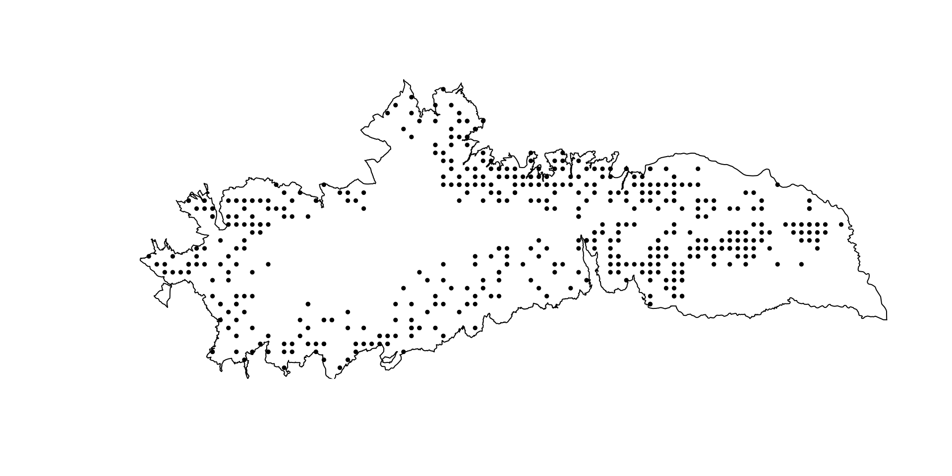
Importar datos vectoriales: Capas disponibles
- Algunos objetos espaciales pueden contener varias capas
- Explorar las capas existentes con
st_layers
Driver: GPX
Available layers:
    layer_name     geometry_type features fields crs_name
1    waypoints             Point       34     24   WGS 84
2       routes       Line String        0     12   WGS 84
3       tracks Multi Line String        1     13   WGS 84
4 route_points             Point        0     25   WGS 84
5 track_points             Point    11759     26   WGS 84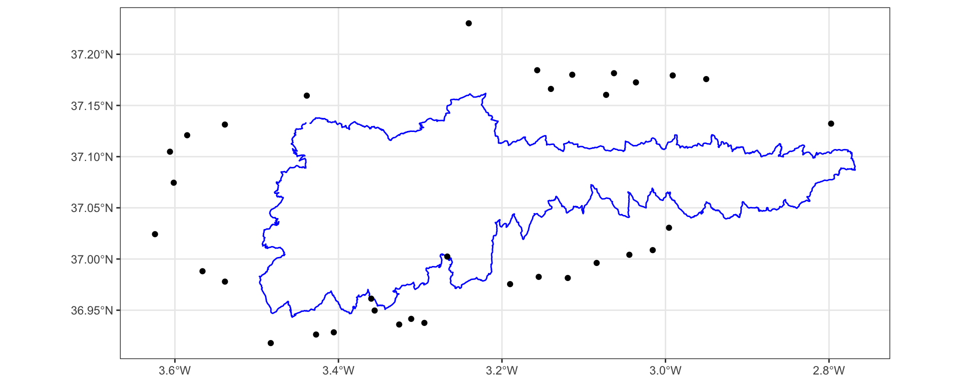
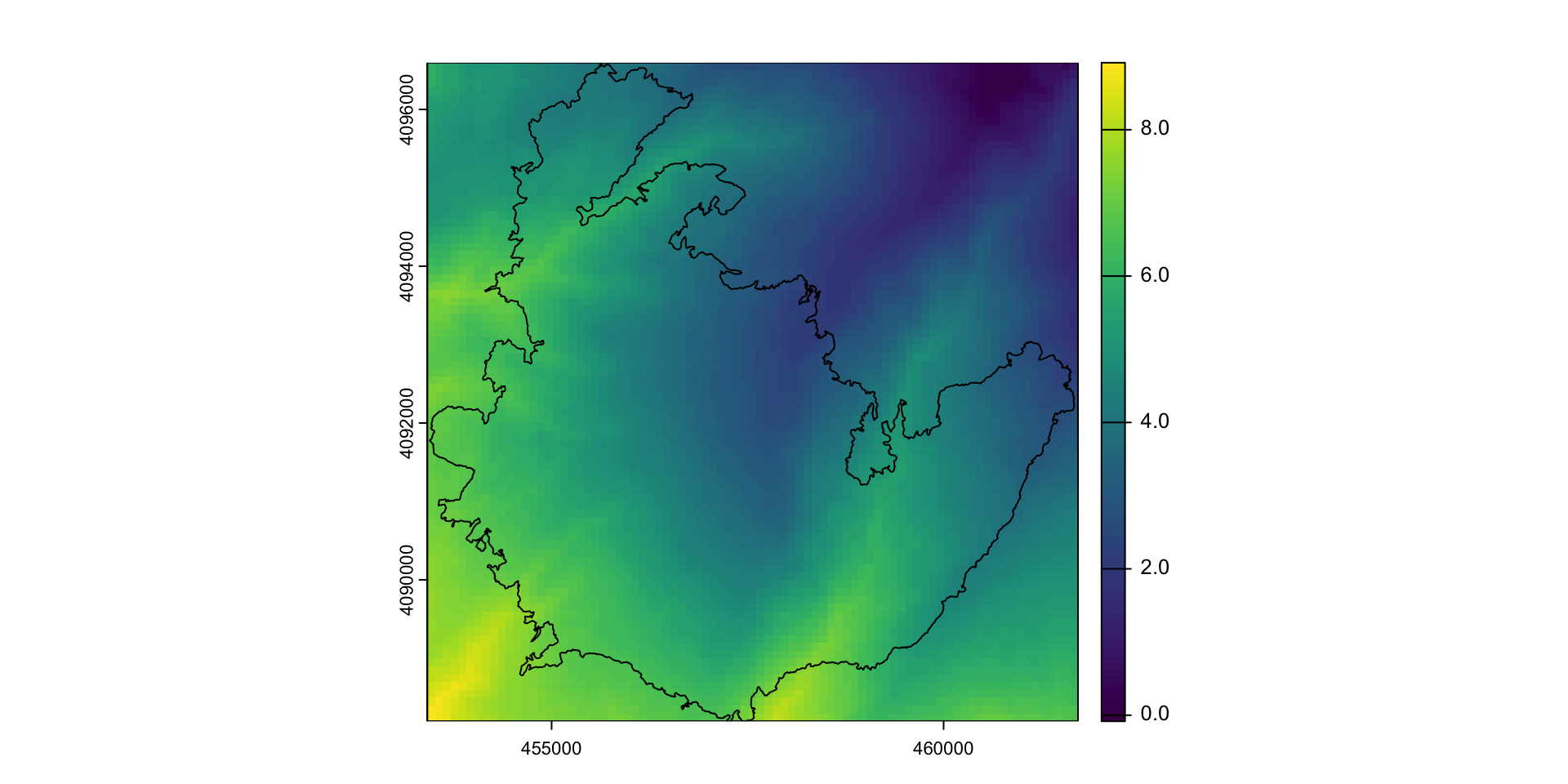
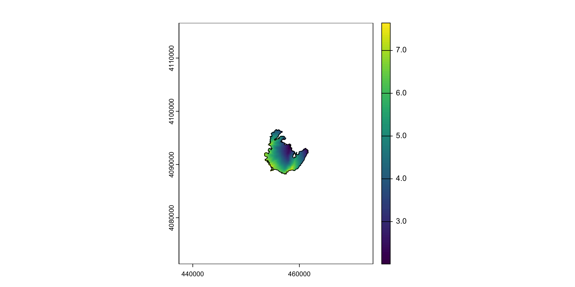
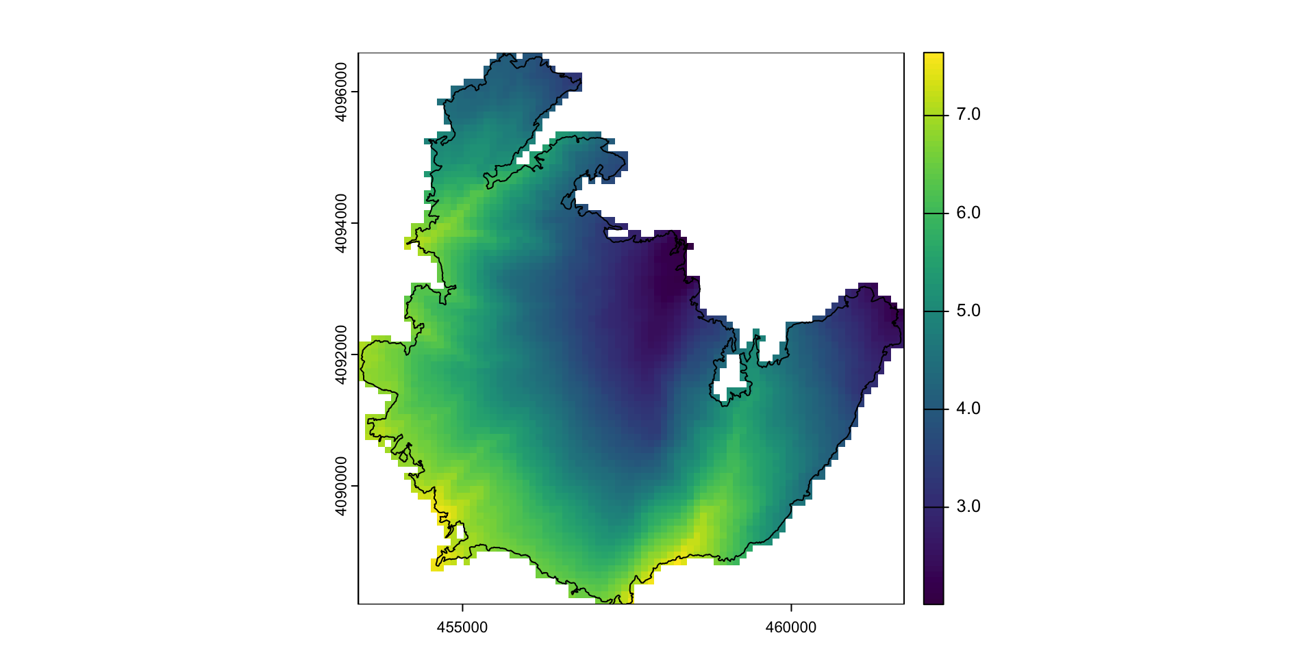
Ráster
Ráster
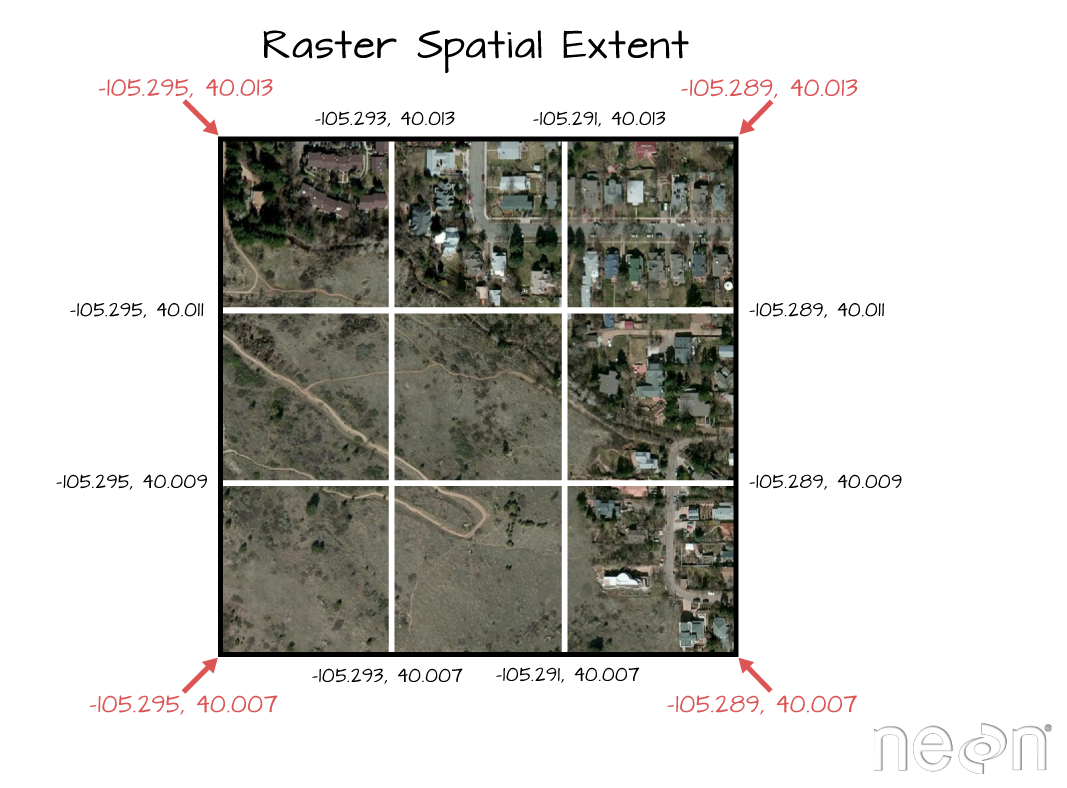
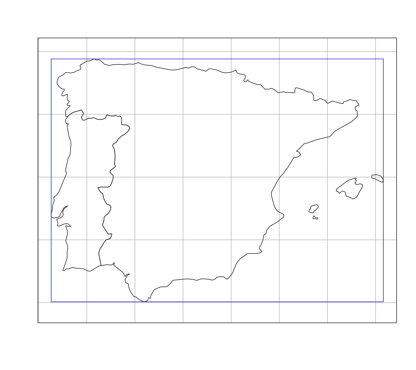
Extensión
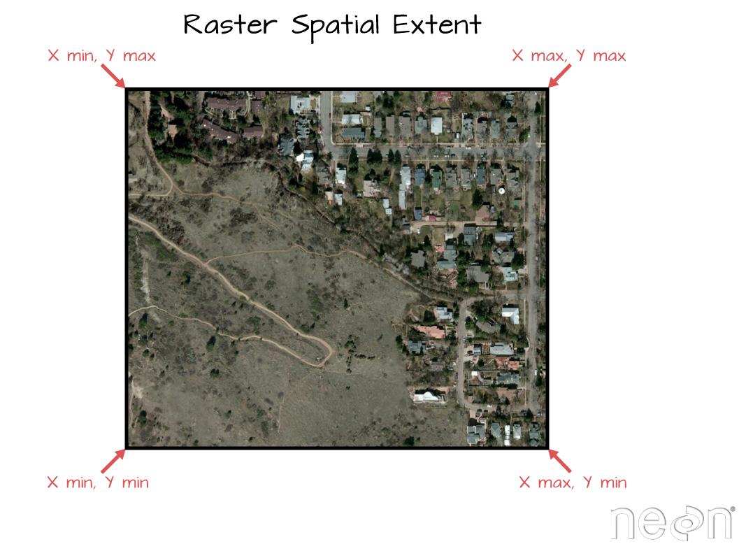
Extensión - Resolución - Sistema de Coordenadas
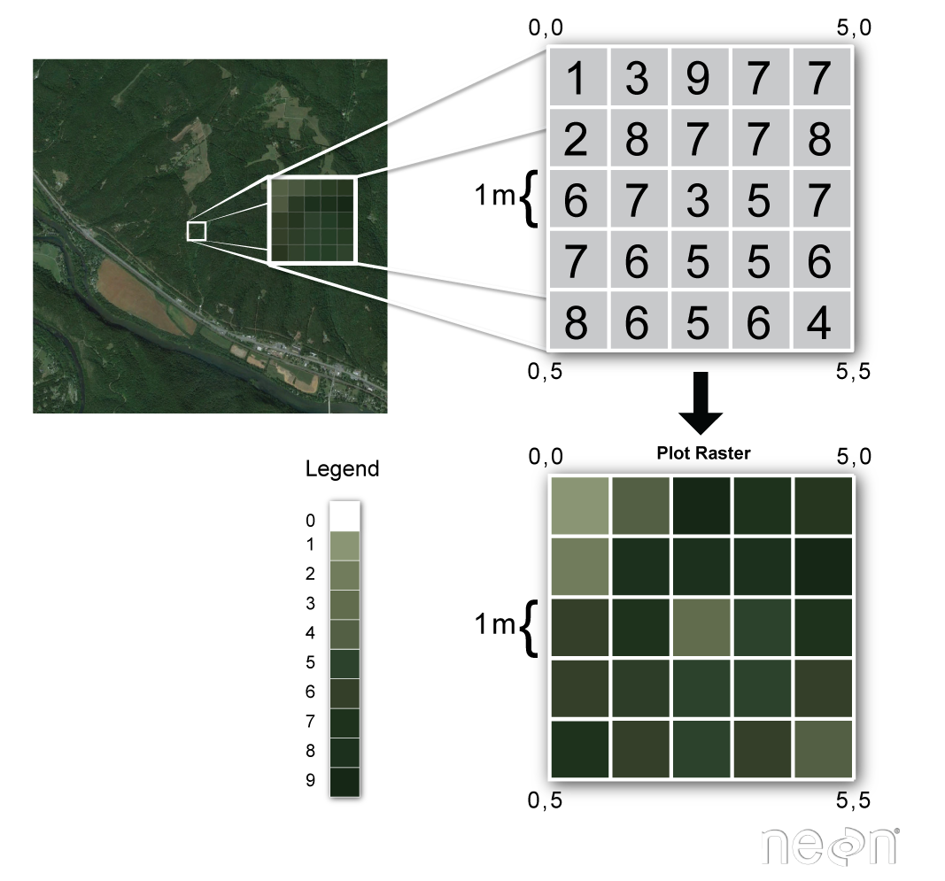
Ejemplo Ráster
library(terra)
my_rast <- terra::rast(here::here("assets/ext_data/geoinfo/tmin_1971_2000_3042.tif"))
my_rast
class : SpatRaster
dimensions : 453, 364, 1 (nrow, ncol, nlyr)
resolution : 100, 100 (x, y)
extent : 437414, 473814, 4071295, 4116595 (xmin, xmax, ymin, ymax)
coord. ref. : ETRS89 / UTM zone 30N
source : tmin_1971_2000_3042.tif
name : tmin_1971_2000
min value : -1.647195
max value : 12.123637 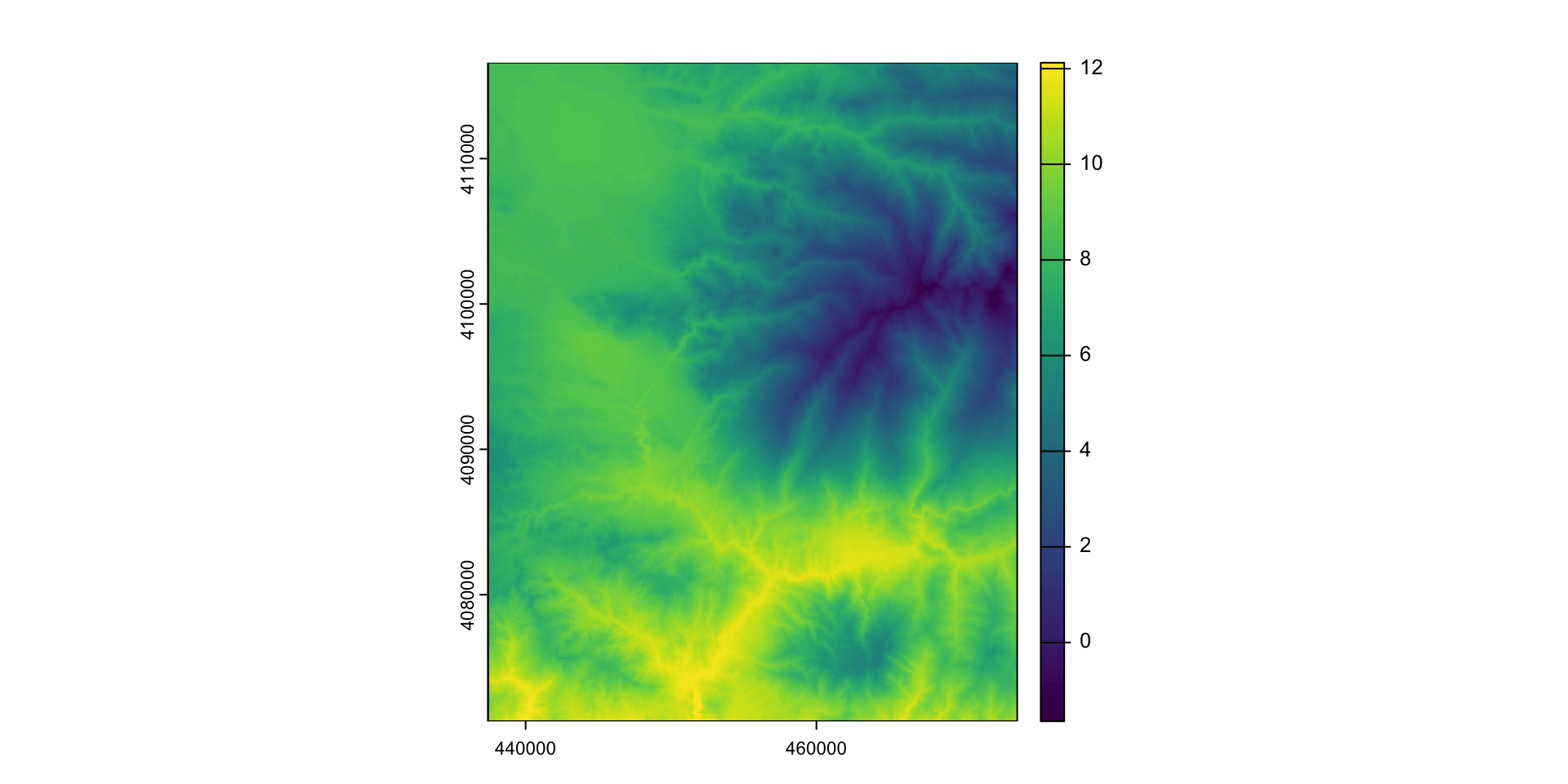
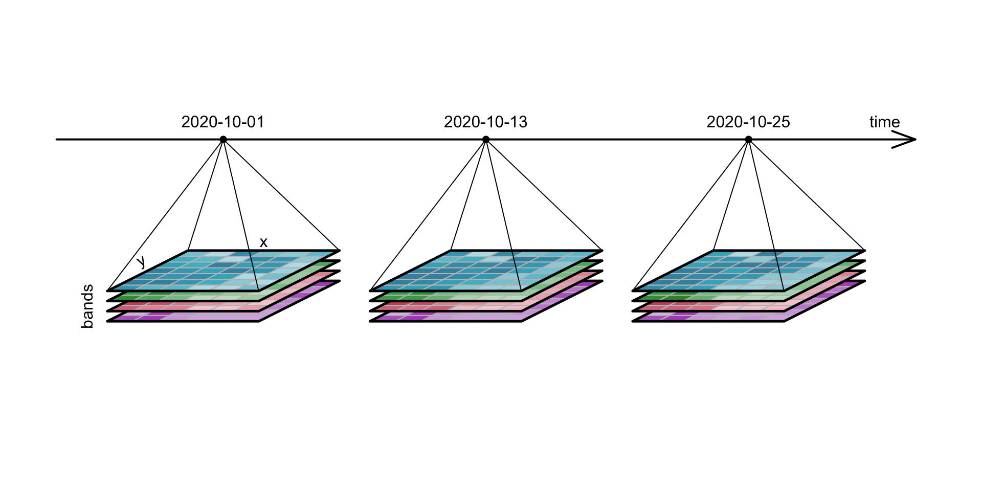
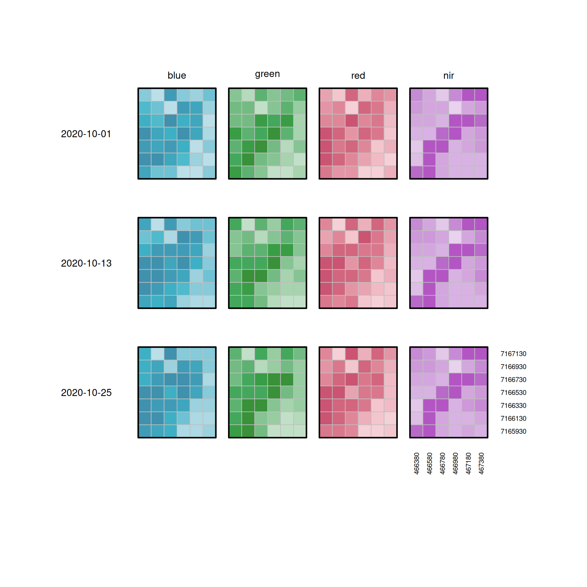
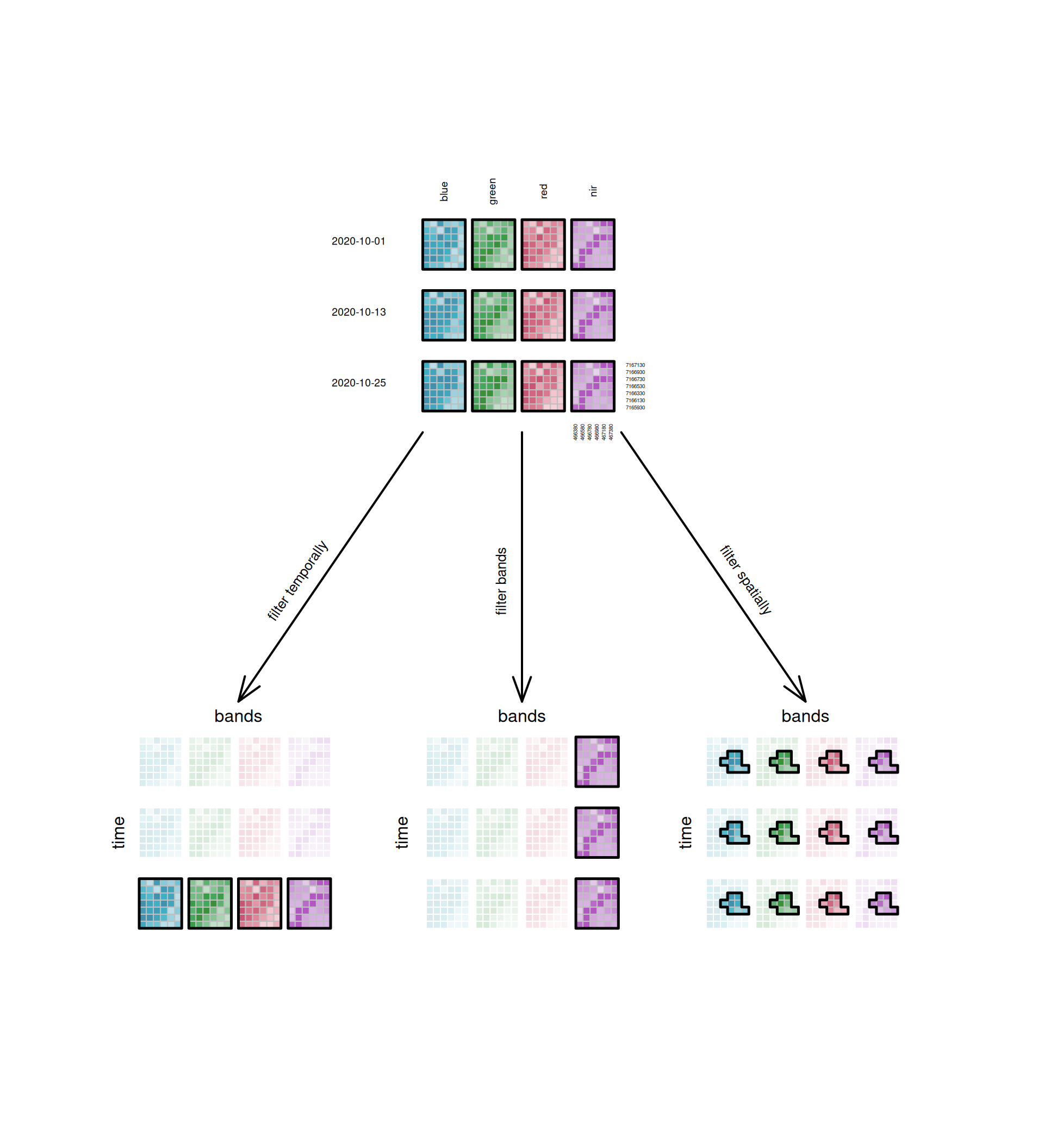
Stacks
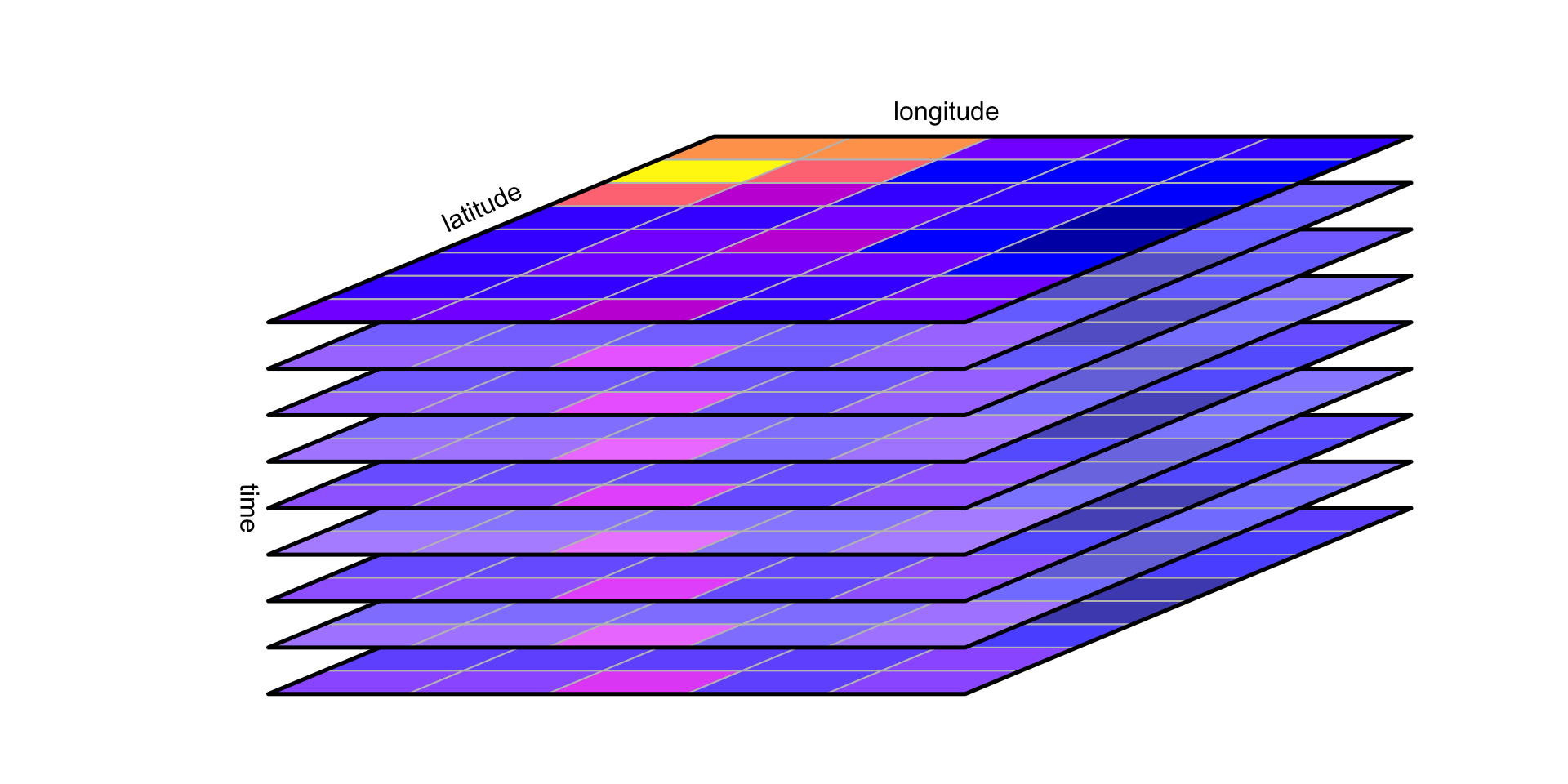
Fuente: Pebesma & Bivand (2025)
Data cubes
Bounding box
Code
library(sf)
library(dplyr)

# Crear polígonos irregulares distribuidos más aleatoriamente
encinar_1 <- st_polygon(list(rbind(c(1,5), c(2.3,4.2), c(3.2,5.6), c(3,7), c(2.1,7.5), c(1.3,7), c(0.7,5.8), c(1,5))))
encinar_2 <- st_polygon(list(rbind(c(7,2), c(8.5,1.1), c(9.6,2.3), c(9.2,3.9), c(8.4,4.4), c(7.6,4.1), c(7.1,2.8), c(7,2))))
robledal_1 <- st_polygon(list(rbind(c(3,8), c(4.7,7.1), c(5.4,8.5), c(5.1,9.6), c(4.3,10.3), c(3.5,9.9), c(3.1,8.8), c(3,8))))
robledal_2 <- st_polygon(list(rbind(c(8,6), c(9.9,5.0), c(10.8,7.1), c(10.2,8.5), c(9.1,9.3), c(8.2,7.8), c(8,6))))
pinar <- st_polygon(list(rbind(c(4,4), c(6.1,2.8), c(7,5), c(6.5,6.5), c(5.6,6.0), c(4.8,4.6), c(4,4))))


manchas <- st_sf(
  nombre = c("Encinar A", "Encinar B", "Robledal A", "Robledal B", "Pinar"),
  tipo = c("Encinar", "Encinar", "Robledal", "Robledal", "Pinar"),
  geometry = st_sfc(encinar_1, encinar_2, robledal_1, robledal_2, pinar),
  colores = c("darkgreen", "darkgreen", "gold", "gold", "green"),
  crs = 4326
)

manchas <- st_transform(manchas, 23030)

plot(manchas["tipo"], col = manchas$colores, graticule = TRUE, axes = TRUE)
legend("bottomleft", legend =  unique(manchas$tipo),
       fill = unique(manchas$colores), title = "Tipo de Manchas")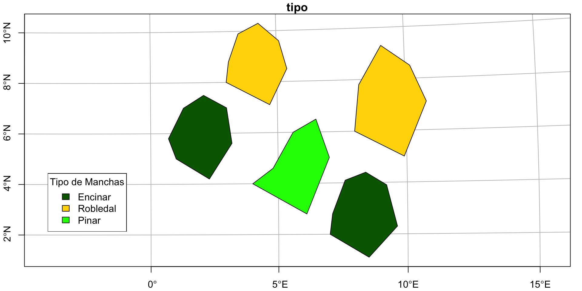
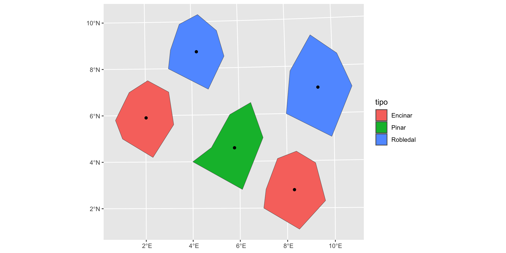
Selección espacial
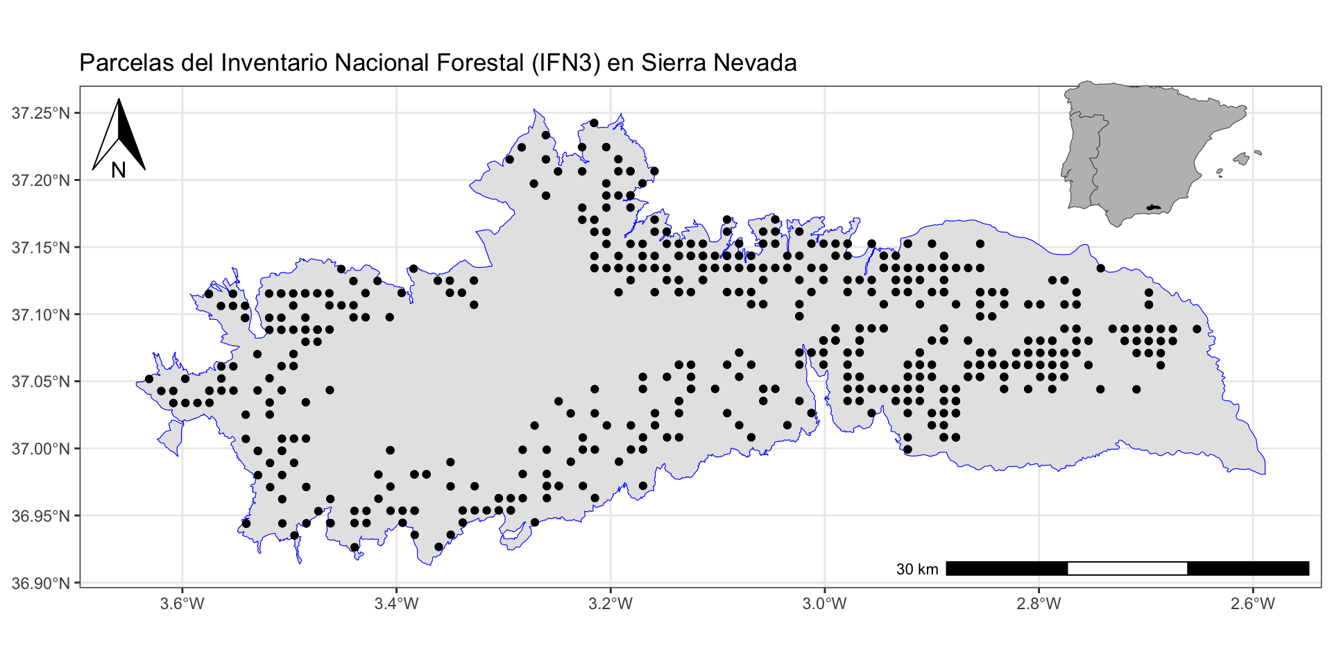
Unión de atributos: visualización
Code
library(ggspatial)

ggplot() +
  geom_sf(data = sn, color = "blue", size = 1) +
  geom_sf(data = ifn_sn_geo_riqueza, aes(size = riqueza)) +
  annotation_north_arrow(location = "topleft",
                         width = unit(1, "cm")) +
  annotation_scale(location = "br", width_hint = 0.3) +
  theme_bw() +
  ggtitle("Parcelas del Inventario Nacional Forestal (IFN3) en Sierra Nevada")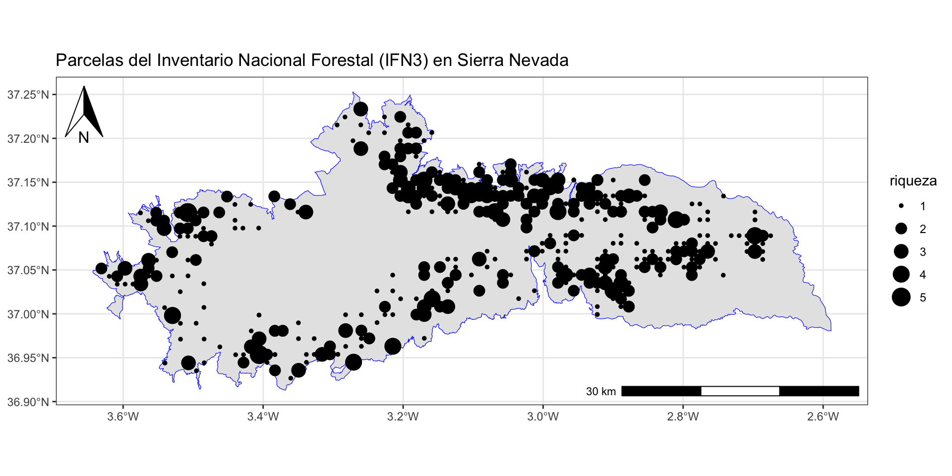
(Extra) Uniones de datos tabulares
Visualización de mapas
Code
library(ggspatial)

mapa<- ggplot() +
  geom_sf(data = sn, color = "blue", size = 1) +
  geom_sf(data = ifn_sn_geo) +
  annotation_north_arrow(location = "topleft",
                         width = unit(1, "cm")) +
  annotation_scale(location = "br", width_hint = 0.3) +
  theme_bw() +
  ggtitle("Parcelas del Inventario Nacional Forestal (IFN3) en Sierra Nevada")
mapa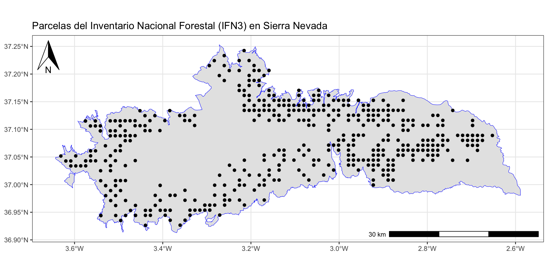
Visualización de mapas
Visualización de mapas
Operaciones básicas con raster
¿Alguna duda?
Ayuda JDC2022-050056-I financiada por MCIN/AEI /10.13039/501100011033 y por la Unión Europea NextGenerationEU/PRTR
![]()
Si usas esta presentación puedes citarla como:
Pérez-Luque, A.J. (2025). Introducción a los SIG con R. Material Docente de la Asignatura: Ciclo de Gestión de los Datos. Master Universitario en Conservación, Gestión y Restauración de la Biodiversidad. Universidad de Granada. https://ecoinfugr.github.io/ecoinformatica/